Understanding similarity or semantic search and vector databases
In an era marked by data explosion, understanding how to effectively search through vast, unstructured data sets is crucial. This article presents a comprehensive overview of similarity or semantic search and vector databases—key technologies driving today's data retrieval systems. We delve into the underlying mechanisms that enhance the precision and relevance of search results, helping you grasp these complex principles in a straightforward manner.
"Similarity search" or "semantic search" refers to finding information that has similar features or meaning from a set of data. It's like searching for similar movies in an app, looking for similar shoes on an e-commerce website, or finding data related to a specific meaning.
At its core, similarity search involves three main aspects: creating vector embeddings, calculating similarity, and optimizing search.
Creating Vector Embeddings
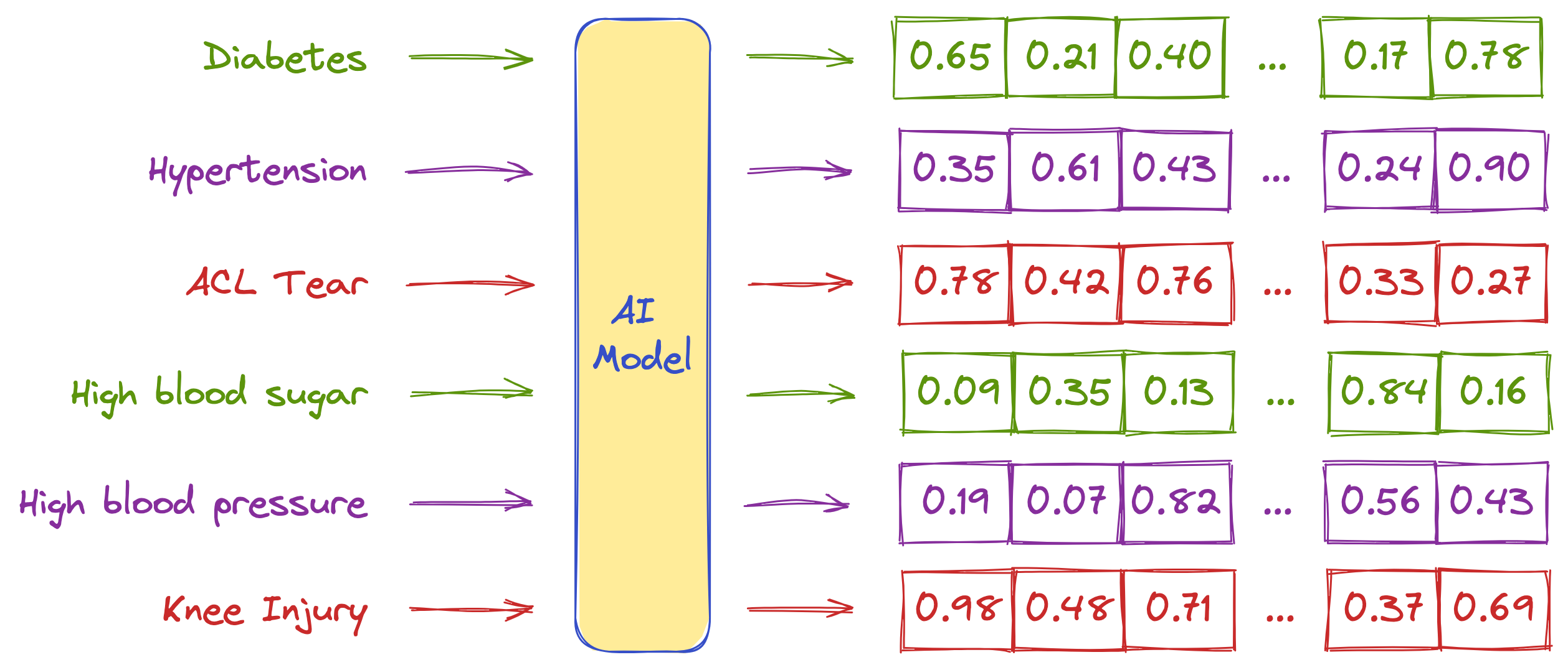
In order to identify similarities or semantics, data items are represented using a specific data structure called "vectors" or “vector embeddings”. Here's what these vectors look like.

These vector embeddings, which come in different sizes, are generated by various systems for different use cases. AI models such as GPT, BERT, or T5 Large Language Models (LLM) generate these embeddings from given text inputs. AI models such as DALL-E generate these embeddings from given images. Alternatively, you can create these embeddings using your own specialized AI processes.
Here is an example of how vector embeddings can be represented when created using an AI model for given text:
If we attempt to visualize the embedding vectors, this is how they would appear in a 3D space.
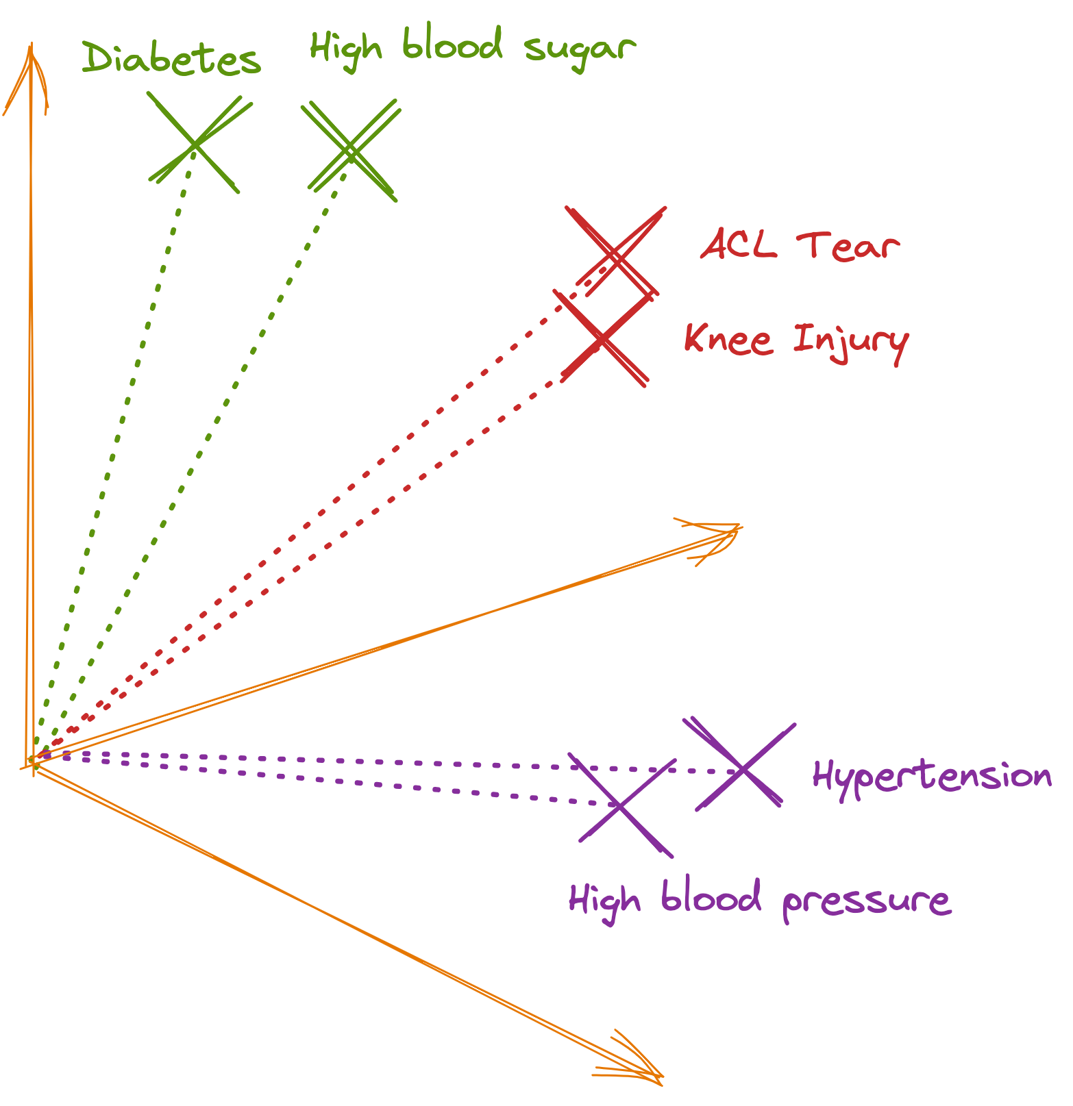
The important aspect of generated embeddings is that similar or semantically related data tend to be located closer to each other, while dissimilar data are located farther apart. This is because AI models are trained on data that helps them identify meanings, similarities, and differences.
To achieve better similarity or semantic results for data within a particular domain, it is important to use AI models that are specialized and trained on domain-specific data.
Calculating similarity
Now that we understand how data is represented, we can learn how to find relevant results by calculating the distances between the vector representation of the search query and the existing data.
When performing a search, the first step is to create a vector embedding using the same AI model or process that was used to create the vector embeddings of the data earlier.
The next step is to calculate the distance between the search query vector embedding and the data vector embeddings.
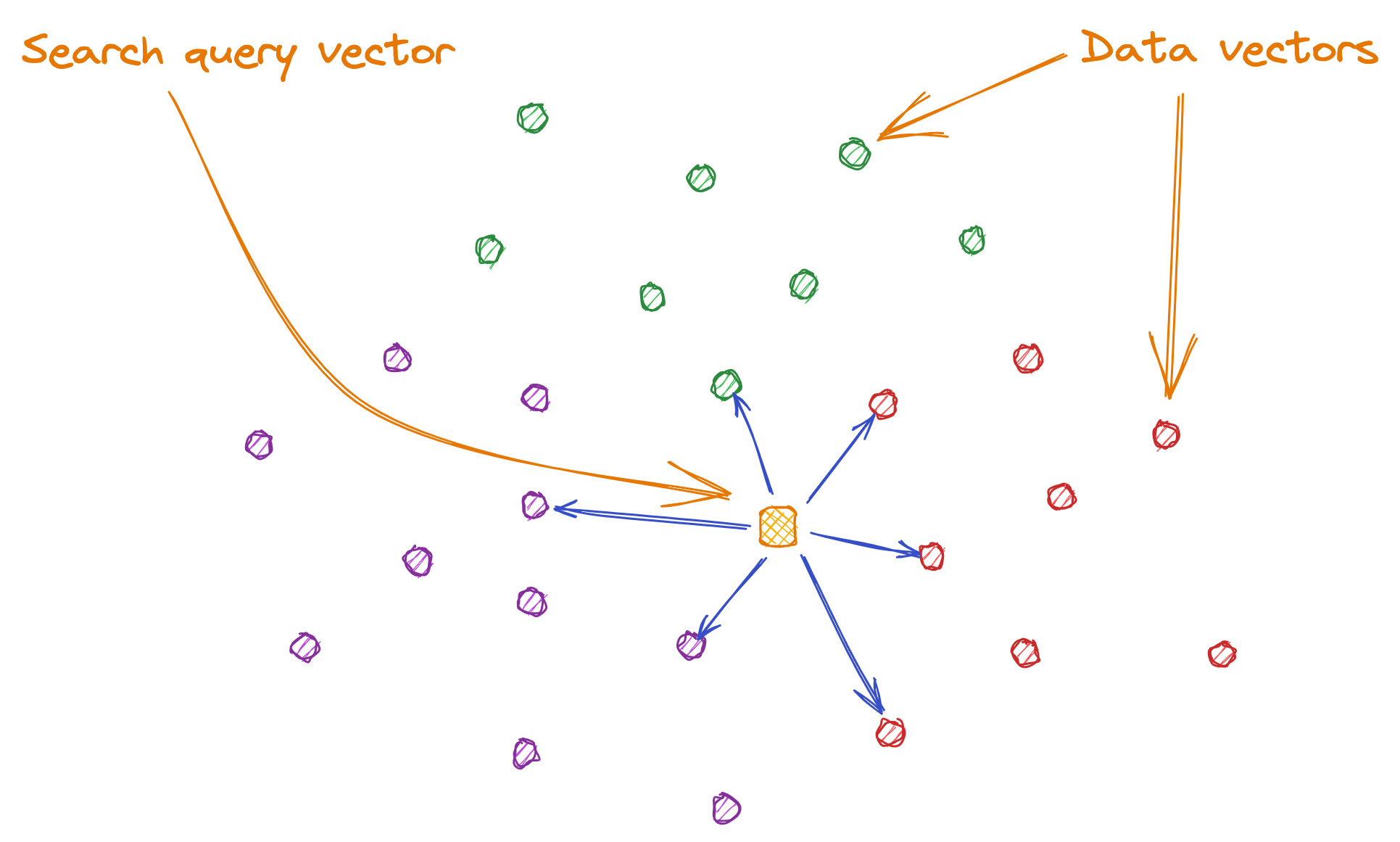
To find potentially similar data vectors to a query vector, we calculate the distance between all data vectors and the query vector.
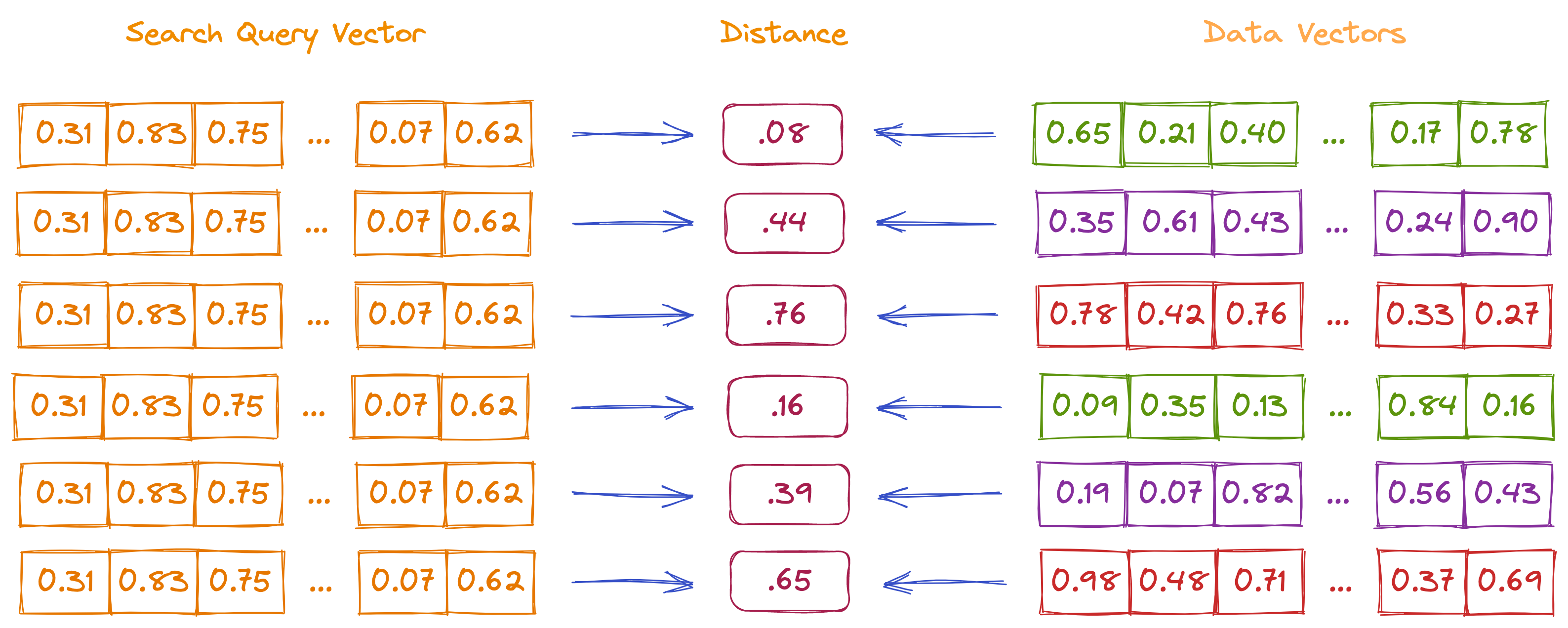
However, not all data is relevant. Therefore, we only need the data vectors that are closest to the query vector, as they are potentially similar. To improve accuracy, we can limit the number of closest vectors to a certain count. When performing a search, the additional information of count or top "K" is provided, which represents the number of closest vectors.
The choice of similarity metric is also a key factor in obtaining more relevant results.
There are multiple ways to calculate the similarity between two vectors. Below are a few widely used similarity metrics as examples.
Euclidean distance (L2)
Essentially, Euclidean distance measures the length of a segment that connects two data points. The smaller the distance between the data points, the more similar they are.
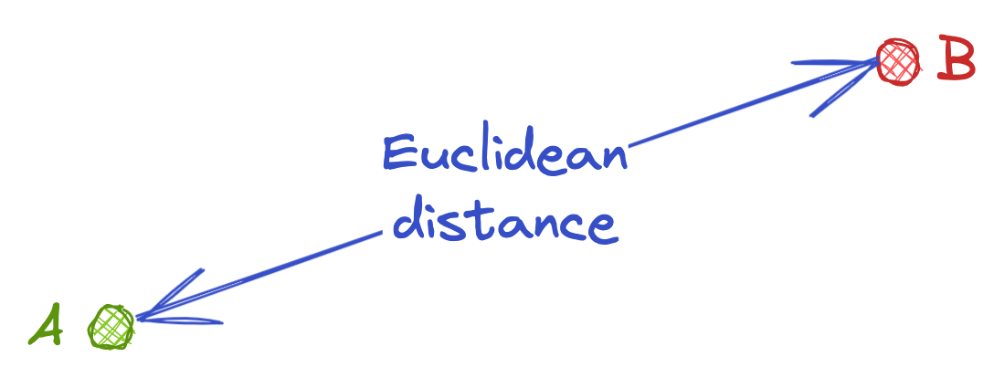
Cosine Similarity or Inner Product (IP)
Cosine similarity measures the angle between two vectors. The smaller the difference between the angles, the more similar the vectors are.
The inner product (IP) of normalized vector embeddings is equivalent to cosine similarity. It is more useful when measuring the orientation but not the magnitude of the vectors.
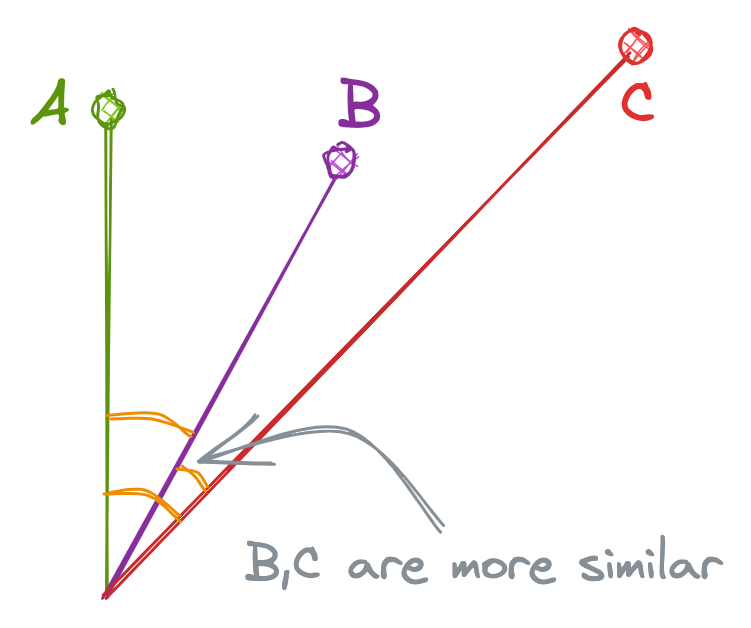
Refer to this to learn more about cosine similarity.
Dot Product (IP)
The Dot Product is mathematically the dot multiplication of 2 vectors. The dot product is proportional to both the cosine and the lengths of vectors. So in the below example, even though the cosine is higher for “B” and “C”, the higher length of “A” makes "A" and "B" more similar than "B" and "C".
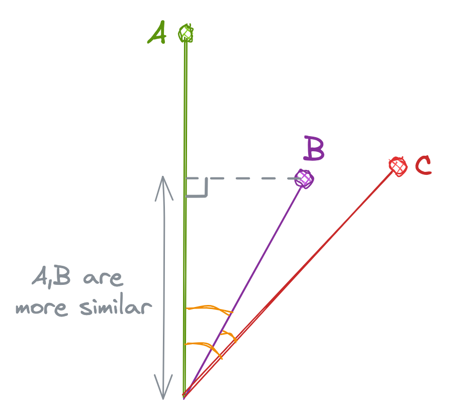
Refer to this to learn more about Dot Product.
Optimizing search
Currently, the similarity is calculated for each data vector against every query vector. This means that if there are one million data vectors, there will be one million similarity calculations, and the most similar data vectors will be returned as the result. However, when dealing with millions or billions of records, this can severely impact performance due to the large number of calculations and memory required.
Optimizing similarity search involves three main factors: search quality, search speed, and system memory required. To achieve this optimization, various algorithms and techniques can be applied, but they come with trade-offs.
One of the most common methods is creating different indexes, which improves the speed of similarity search at the cost of accuracy, while also reducing the required memory. These are known as Approximate Nearest Neighbor (ANN) Search algorithms. Some optimizations are listed below.
Flat Index (No Optimization)
Calculating the similarity of each data vector against every query vector is called "flat" (no optimization). This method is necessary when accuracy is prioritized over other factors.
- Good until 10K - 50K records
- High Accuracy
- Reduced speed when dealing with large amounts of data.
Locality Sensitive Hashing
In this optimization, data records that are near each other are located in the same buckets with high probability, while data points that are far from each other are likely to be in different buckets.
Once the search is performed, the query data is compared against the buckets, and then a specific search is performed within the matched buckets.
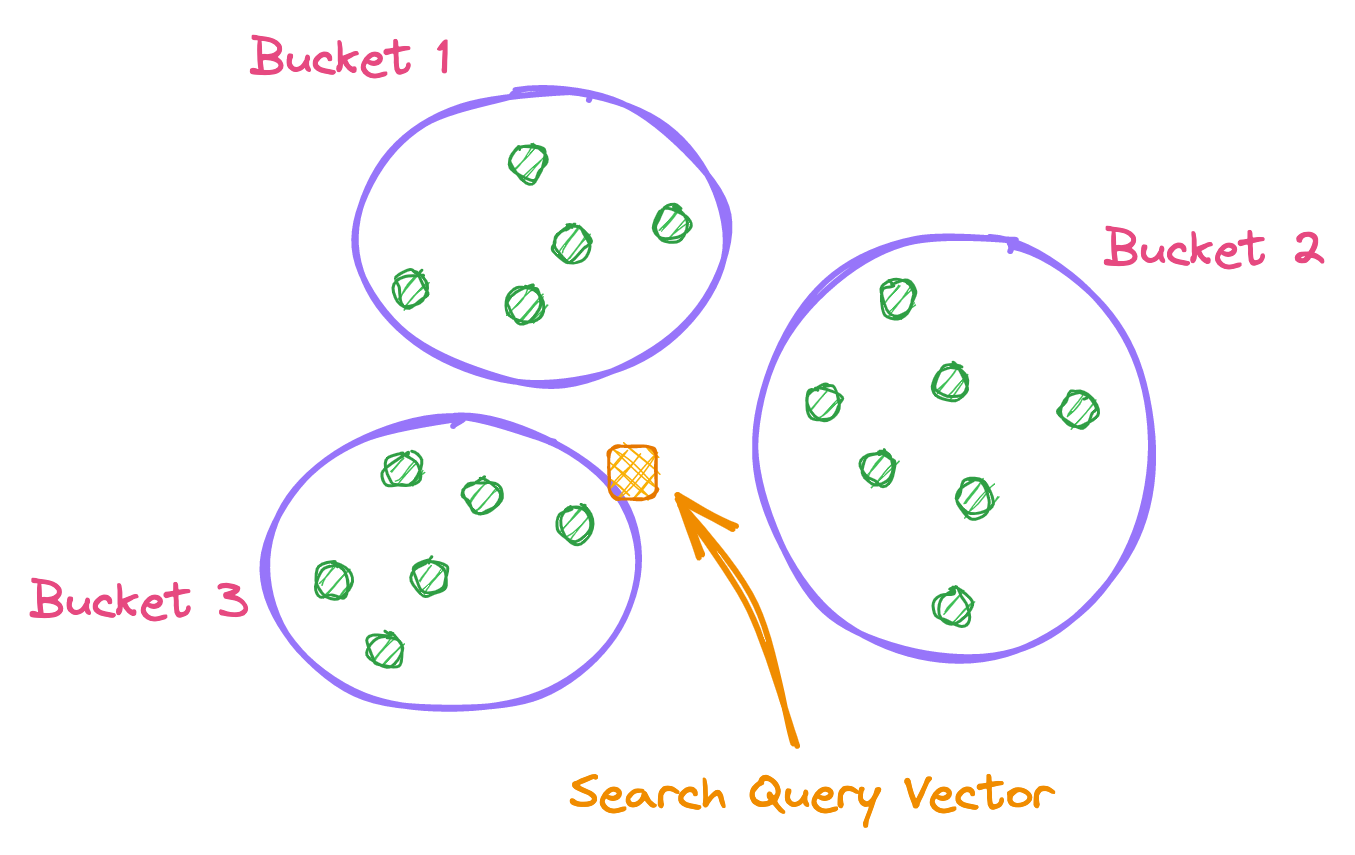
In above example, the search will be performed on Bucket 3 because the query vector is closer to it.
- Moderate Accuracy
- Lot of buckets are required to achieve good results, leading to a lot of extra memory.
Hierarchical Navigable Small World graph (HNSW)
This optimization combines two different methods: 1. Probability Skip List 2. Navigable Small World Graph. It creates a multi-layer graph from the given data, which helps the algorithm quickly find approximate nearest neighbors.
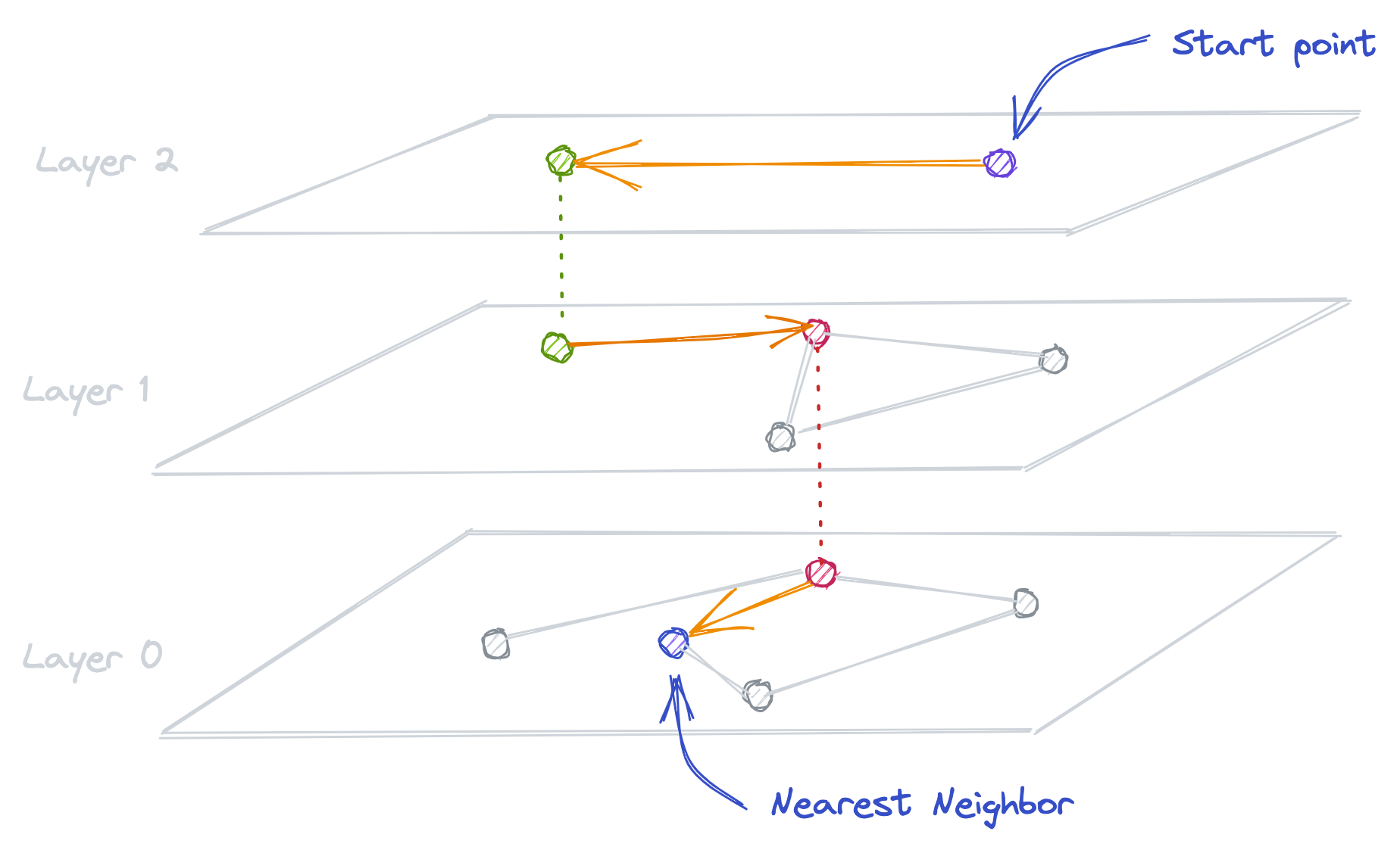
- The accuracy is lower compared to the Flat Index method, but higher compared to other methods.
- Very fast.
- Can work with large datasets.
Product Quantizer (PQ)
Product Quantization (PQ) is a technique for reducing the size of a database by decreasing the overall precision of the vectors.
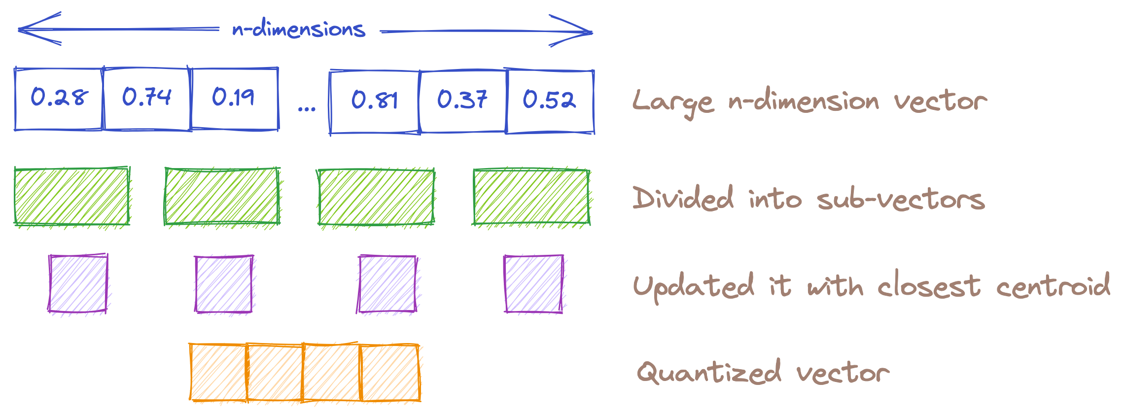
- Less memory is required to search the same dataset compared to other methods.
- Very fast.
- Can work with large datasets.
- Good accuracy.
Inverted file index (IVF)
In this technique the data is partitioned into different cells and associated those partitions with centroid. Cluster centroids are usually determined with a clustering algorithm called k-means. This reduces the overall search scope by arranging the entire dataset into partitions. Because of this only a fraction of the database is compared to the query.
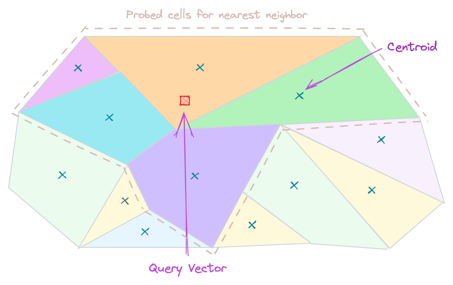
- Good Accuracy
- Less memory required
- Average speed compared to other optimizations.
Vector Databases
The preceding discussion focused on the core aspects of similarity search. What vector databases offer is an infrastructure for those algorithms, providing capabilities such as scalability, high availability, APIs for adding/updating/deleting data, and other integrations.
"Vector Database" is not technically a database; rather, it is a search tool for similarity, similar to other search tools such as "ElasticSearch", "Algolia", or "Typesense". Typically, I reserve the term "database" for systems where the data stored in it is the primary source of truth, such as "MySQL", "PostgreSQL", or "MongoDB". "Vector Databases" are not the primary source of truth for the system.
Vector databases use the aforementioned search optimization techniques in different combinations to improve both speed and accuracy.
There are multiple vector databases in the market. Each one has its pros and cons.:
Nowadays, existing search engines and databases also started supporting vector search.
As the volumes of unstructured data continue to surge, these technologies will persist in their evolution. Scalability, computational efficiency, and precision will remain at the forefront of this evolution.
In the next article, let's explore how we can implement and deploy our own vector search engine.